Learning the parameters of a predictive model and testing it on the same data is a methodological mistake: a model that would just repeat the labels of the samples that it has just seen would have a perfect score but would fail to predict anything useful on yet-unseen data. This situation is called overfitting. To avoid it, it is common practice when performing a (supervised) machine learning experiment to hold out part of the available data as a test set.
This is called validation: a set of techniques used to make sure a predictive model performs well in a wide range of situations, and is not just optimised for a particular dataset or set of conditions. In this section I cover 2 of the more widely used validation methods describing some of the issues and how these can be overcome.
Train Test Split
Train test split is a validation method that partitions the original dataset into a training set to train the model; a validation set for tuning the model; and a test set to evaluate it. There is no general rule dictating how many samples should be made available for each set and depends largely and how strong the patterns are in the data. However it is advised to maximise the training data as much as possible.
The training set, as the name suggests, is used to train a predictive model by attempting to identify the patterns in the data that drive it to generalise on a solution. During training the model fits itself around the data it is provided, but there is no validation performed at this stage.
The validation set is used strictly for model tuning. Using the model created during training, parameters may be tuned and the performance of each adjustment is recorded. Using an independent dataset attempts to prevent the model from “cheating” and inaccurately reporting higher performance for a particular combination of parameter values.
The test set is used to make a final estimate of the error. Until this point, the most performant model has been exposed to both the training and validation sets for parameter tuning. So, it must be checked on an unseen set so that we may forecast how well it will perform in the real world.
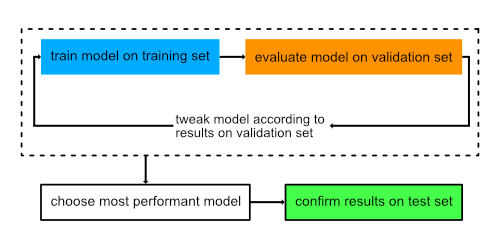
We can see how the Enron dataset may be split to create a training, validation,
and test set using
train_test_split.
Note that the dataset is shuffled to distribute the class labels.
from sklearn.model_selection import train_test_split

# First shuffle the data.
shuffled_data = enron_data.sample(frac=1).reset_index(drop=True)

# Create a 80% split of the data.
split_boundary = int(len(shuffled_data) * .80)
test_set = shuffled_data[split_boundary:]
train_validation_set = shuffled_data[:split_boundary]

# Create a further split for training and validation data.
X_train, X_valid, y_train, y_valid = train_test_split(
  train_validation_set.drop(columns=['poi']),
  train_validation_set['poi'],
  test_size=0.25,
  random_state=42
)

# Justify the output of samples.
print_samples = lambda t, samples: print('{} set:'.format(t).ljust(16), len(samples), 'samples')

print_samples('training', X_train)
print_samples('validation', X_valid)
print_samples('test', test_set)
training set:    83 samples
validation set:  28 samples
test set:        28 samples
The above however is only viable when there is enough data to make three splits. In this example I have created a 60-20-20 split that yields only 83 samples from the Enron dataset to be used for training. This is likely not nearly enough data to identify patterns that are possibly hidden in the other 56 samples being used for validation and testing. Furthermore making such a segregation, despite the data having been shuffled, may disturb the target distribution and therefore we may find that most of the persons of interest are contained in any one of the three sets.
This is one of the drawbacks of this particular validation strategy and by definition it does not maximise the number of samples available for training since it must hold back a percentage of the samples to be distributed across both the validation and test sets.
On a more general note validation and test sets “wear out” with repeated use. That is, the more you use the same data to make decisions about hyperparameter settings or other model improvements, the less confidence you’ll have that these results actually generalize to new, unseen data. Note that validation sets typically wear out more slowly than test sets.
If possible, it’s a good idea to collect more data to “refresh” the validation and test sets. This of course is not possible in respect to the Enron dataset since we already have the records of all employees at the company.
Cross-validation
Cross-validation is a technique to validate predictive models by partitioning the original dataset into a training set to train the model, and a test set to evaluate it.
In k-fold cross-validation, the original sample is randomly partitioned into k
equal size subsamples. Of the k subsamples, a single subsample is retained as
the validation data for testing the model, and the remaining k-1 subsamples
are used as training data. The cross-validation process is then repeated k
times (the folds), with each of the k subsamples used exactly once as the
validation data. The k results from the folds can then be averaged (or
otherwise combined) to produce a single estimation.
Moreover, we can use the
StratifiedShuffleSplit
cross-validation object; a merge of
StratifiedKFold
and
ShuffleSplit,
which returns stratified randomised folds. The folds are made by preserving the
percentage of samples for each class.
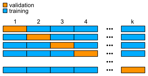
As before we can see how this may be applied to the Enron dataset using the object sklearn.
from sklearn.model_selection import StratifiedShuffleSplit

# Cross-validator with 10 splits.
cv = StratifiedShuffleSplit(n_splits=10, test_size=0.1)

# The cross-validator returns an iterator. Grab only the first item.
X_train, X_valid = next(cv.split(enron_data.drop(columns=['poi']), enron_data['poi']))

# Justify the output of samples.
print_samples = lambda t, samples: print('{} set:'.format(t).ljust(16), len(samples), 'samples')

print_samples('training', X_train)
print_samples('validation', X_valid)
training set:    125 samples
validation set:  14 samples
The advantage of this method is that all samples are used for both training and validation, and each sample is used for validation exactly once. This therefore maximises the number of samples used for training.
For the remainder of this experiment I shall use cross validation when evaluating my models and their respective hyperparameters.
Testing
To drive the evaluation of each classifier I will use the function included in
this project, test_classifier, offering a consistent means through which every
classifier may be tested. Furthermore it will be the same function used to
evaluate my classifier upon submission.
from tester import test_classifier
This testing strategy does however come with the limitation that I am unable to manipulate the validation data before it is used to evaluate each classifier. This is something I discussed earlier concerning validation leakage. If this were not the case I could perform imputation at the time of evaluation such that the validation set is not biased by the same data used for training.
Using the above function I have additionally implemented a means through which to test multiple classifiers sequentially whilst keeping the output to a minimum. Once each classifier has been tested the results are returned in a DataFrame and the results sorted (ascending F1 score by default). This is really useful to reduce the noise in this notebook, displaying only the most important information.
from utils import redirect_stdout

def test_classifiers(clfs, dataset, features, sort_by='f1', verbose=False):
  results = pd.DataFrame(columns=['accuracy', 'precision', 'recall', 'f1', 'f2'])
  for _, (name, clf) in enumerate(clfs):
    print('=====> Running {}\n'.format(name))
    if verbose:
      results.loc[name] = test_classifier(clf, dataset, features)
    else:
      with redirect_stdout():
        results.loc[name] = test_classifier(clf, dataset, features)
  return results.sort_values(by=sort_by, ascending=False)