In previous sections I’ve cleaned data that exhibited issues with data entry and missing values. Now I would like to discover the outliers. This part of the data exploration has deliberately been left until last. The reason being that this step is destructive. That is up until now we have been correcting the data so that it is true to the source, or using sensible data where it was otherwise not available. In this section I will remove data that will not be useful to the investigation.
Conveniently the definition of an outlier can be described as a point which falls more than 1.5 times the interquartile range above the third quartile or below the first quartile.
original_data = enron_data.drop(columns=['poi']) # poi is not a feature and should not be considered

first_quantile = original_data.quantile(.25)
third_quantile = original_data.quantile(.75)

median = original_data.quantile(.5)
interquantile_range = third_quantile - first_quantile

outlier_data = median + 1.5 * interquantile_range
outliers = (original_data > outlier_data).sum(axis=1).to_frame(name='# of outliers') \
    .sort_values('# of outliers', ascending=False)

five_percent_of_sample = int(len(enron_data) * 0.06)

# Merge the outliers with the original enron data.
outliers = outliers.merge(right=enron_data, how='inner', left_index=True, right_index=True) \
  .loc[:, ['# of outliers', 'poi']]
outliers.head(five_percent_of_sample)
| # outliers | poi | |
|---|---|---|
| FREVERT MARK A | 13 | False |
| LAY KENNETH L | 13 | True |
| SKILLING JEFFREY K | 12 | True |
| TOTAL | 12 | False |
| WHALLEY LAWRENCE G | 12 | False |
| LAVORATO JOHN J | 10 | False |
| HAEDICKE MARK E | 8 | False |
| BELDEN TIMOTHY N | 8 | True |
Our data set is really small, so I’m going to consider just 5% of the samples with the largest number of outliers:
- Mark Frevert and Lawrence ‘Greg’ Whalley are lesser known employees but still top managers of Enron (the latter being President and COO of Enron) who also represent valuable examples for our predictive model.
- Kenneth Lay (Enron chairman and CEO) and Jeffrey Skilling (former Enron president and CEO) are very well known persons from Enron and heavily involved in the scandal. They represent important examples in our dataset and falsely flagged as true outliers.
- The example TOTAL is the total value of financial payments from the FindLaw dataset. This clearly is not an individual person and will unbalance the distribution across several features in the dataset. Therefore it should be removed.
- John Lavorato, another senior Enron executive, has little media exposure and there are no reports of him being involved in the scandal. Since his data contains many outliers that could potentially bias our predictive model I’ll remove him from the dataset.
- Timothy ‘Norris’ Belden is the former head of trading in Enron Energy Services. He is considered a key player in the Enron scandal constituting a good example for our predictive model.
From the above considered 8 examples I will exclude only 2 of them. However before doing so I will visualise some of the features, hoping they will make the outliers and errors immediately stand out. This will convince me further that these examples should be removed from the dataset.
from ggplot import *

ggplot(enron_data, aes(x='salary', y='bonus', color='poi')) + \
  geom_point(size=40.0)
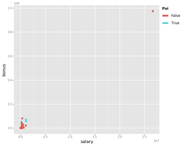
The above graph diagrams the salaries each Enron employee earned against the bonuses they received. It is evident that there is some discrepancy with this data where one employee received both a salary and bonus at a size well beyond everyone else. Let’s take a look at this data point more closely.
enron_data[enron_data['salary'] > 1e7]
| salary | to_messages | deferral_payments | total_payments | exercised_stock_options | bonus | restricted_stock | shared_receipt_with_poi | restricted_stock_deferred | total_stock_values | expenses | loan_advances | from_messages | other | from_this_person_to_poi | poi | directors_fees | deferred_income | long_term_incentive | from_poi_to_this_person | |
|---|---|---|---|---|---|---|---|---|---|---|---|---|---|---|---|---|---|---|---|---|
| TOTAL | 26704229.00 | 944.00 | 32083396.00 | 309886585.00 | 311764000.00 | 97343619.00 | 130322299.00 | 594.00 | -7576788.00 | 434509511.00 | 5235198.00 | 83925000.00 | 41.00 | 42667589.00 | 6.00 | False | 1398517.00 | -27992891.00 | 48521928.00 | 26.50 |
This data point corresponds to the TOTAL flagged previously as an outlier.
Let’s just remove this and make the same plot to see how things have improved.
enron_data = enron_data.drop('TOTAL')

ggplot(enron_data, aes(x='salary', y='bonus', color='poi')) + \
  geom_point(size=40.0)
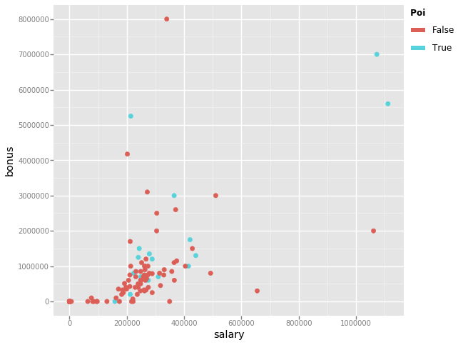
You may conclude that there are four more outliers in the data. However considering the top 2 earners are Jeffrey Skilling and Kenneth Lay, both persons of interest, these should remain in the dataset. Similarly we can conclude there to be a single outlier within the bonus data. We can list the highest receivers to see just who this is.
enron_data.sort_values(by='bonus', ascending=False).head().loc[:, ['salary', 'bonus', 'poi']]
| salary | bonus | poi | |
|---|---|---|---|
| LAVORATO JOHN J | 339288.00 | 8000000.00 | False |
| LAY KENNETH L | 1072321.00 | 7000000.00 | True |
| SKILLING JEFFREY K | 1111258.00 | 5600000.00 | True |
| BELDEN TIMOTHY N | 213999.00 | 5249999.00 | True |
| ALLEN PHILLIP K | 201955.00 | 4175000.00 | False |
The person receiving the highest bonus is John Lavorato, somebody we have already identified above as a potential outlier. Given this name has appeared a couple times as an outlier I will remove it from the dataset.
enron_data = enron_data.drop('LAVORATO JOHN J')

ggplot(enron_data, aes(x='salary', y='bonus', color='poi')) + \
  geom_point(size=40.0)
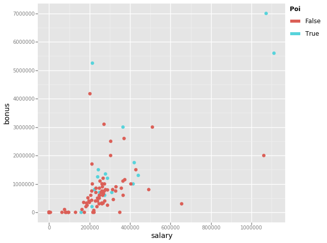
Now that we’ve cleaned up the dataset, lets see how many examples and features remain.
enron_data.info()

<class 'pandas.core.frame.DataFrame'>
Index: 139 entries, ALLEN PHILLIP K to YEAP SOON
Data columns (total 20 columns):
salary                       139 non-null float64
to_messages                  139 non-null float64
deferral_payments            139 non-null float64
total_payments               139 non-null float64
exercised_stock_options      139 non-null float64
bonus                        139 non-null float64
restricted_stock             139 non-null float64
shared_receipt_with_poi      139 non-null float64
restricted_stock_deferred    139 non-null float64
total_stock_value            139 non-null float64
expenses                     139 non-null float64
loan_advances                139 non-null float64
from_messages                139 non-null float64
other                        139 non-null float64
from_this_person_to_poi      139 non-null float64
poi                          139 non-null bool
director_fees                139 non-null float64
deferred_income              139 non-null float64
long_term_incentive          139 non-null float64
from_poi_to_this_person      139 non-null float64
dtypes: bool(1), float64(19)
memory usage: 21.9+ KB
In total I have:
- removed 7 examples,
- removed 1 feature,
- corrected inconsistent data,
- filled in missing financial data with a zero value,
- imputed missing email data using the median value from each class.
Let’s write this cleaned dataset to disk to be used for the later evaluation.
# Save the cleaned dictionary containing the dataset.
with open('final_prject_dataset_cleaned.pkl', 'wb') as data_file:
    pickle.dump(enron_data.to_dict(orient='index'), data_file, protocol=pickle.HIGHEST_PROTOCOL)
With the dataset cleaned up it feels about the right time to investigate how machine learning can help identify persons of interest, starting with how the results of the investigation are to be measured, to ensure consistent and fair comparison between alternative approaches. This will be the focus of the next post on theis topic.