Previously we corrected a couple of data entry issues that found their way into the Enron dataset and discussed how this may have otherwise affected the predicting power of our model. This post builds on this work and continues the data exploratory section of this project by addressing missing and incomplete data.
As seen in a previous posts this dataset is plagued with missing values. Using the same Pandas DataFrame we can print out a list of all the features in the dataset alongside the number of values missing for that feature.
missing_data = enron_data.isna().sum().to_frame(name='# missing values')
missing_data
| # missing values | |
|---|---|
| salary | 51 |
| to_messages | 60 |
| deferral_payments | 108 |
| total_payments | 21 |
| exercised_stock_options | 45 |
| bonus | 64 |
| restricted_stock | 35 |
| shared_receipt_with_poi | 60 |
| restricted_stock_deferred | 128 |
| total_stock_value | 20 |
| expenses | 49 |
| loan_advances | 142 |
| from_messages | 60 |
| other | 54 |
| from_this_person_to_poi | 60 |
| poi | 0 |
| director_fees | 130 |
| deferred_income | 96 |
| long_term_incentive | 80 |
| email_address | 35 |
| from_poi_to_this_person | 60 |
From the above we can see that every example in the dataset has a value for
poi, indicating whether it represents a person of interest. However no other
features can be considered complete. This will have the effect of causing
difficulty for our predictive model to discover patterns from this data. The
feature of largest concern is loan_advances which has only 4 values present in
the entire dataset (~3%). Lets visualise the extent of the missing values in the
form of a bar graph.
missing_data.plot(kind='bar', figsize=(15,5));
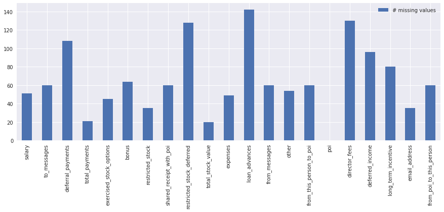
Due to the high number of missing values there may be many examples not offering anything useful to our predictive model. I’ve chosen, somewhat arbitrarily, a threshold of 85% missing values to mean those examples we may be interested in removing from the dataset.
We can retrieve these examples using the following snippet (thank you stackoverflow and Wen).
threshold = .85

# Return the rows that have a percentage of their data missing.
#
# `enron_data.isna().sum(1)` gives the number of missing values for each person.
# `enron_data.shape[1]` is equivalent to `len(enron_data.columns)`
enron_data[(enron_data.isna().sum(1) / enron_data.shape[1]) > threshold]
| salary | to_messages | deferral_payments | total_payments | exercised_stock_options | bonus | restricted_stock | shared_receipt_with_poi | restricted_stock_deferred | total_stock_value | … | loan_advances | from_messages | other | from_this_person_to_poi | poi | director_fees | deferred_income | long_term_incentive | email_address | from_poi_to_this_person | |
|---|---|---|---|---|---|---|---|---|---|---|---|---|---|---|---|---|---|---|---|---|---|
| GRAMM WENDY L | nan | nan | nan | 119292.00 | nan | nan | nan | nan | nan | nan | … | nan | nan | nan | nan | False | 119292.00 | nan | nan | NaN | nan |
| LOCKHART EUGENE E | nan | nan | nan | nan | nan | nan | nan | nan | nan | nan | … | nan | nan | nan | nan | False | nan | nan | nan | NaN | nan |
| THE TRAVEL AGENCY IN THE PARK | nan | nan | nan | 362096.00 | nan | nan | nan | nan | nan | nan | … | nan | nan | 362096.00 | nan | False | nan | nan | nan | NaN | nan |
| WHALEY DAVID A | nan | nan | nan | nan | 98718.00 | nan | nan | nan | nan | 98718.00 | … | nan | nan | nan | nan | False | nan | nan | nan | NaN | nan |
| WROBEL BRUCE | nan | nan | nan | nan | 139130.00 | nan | nan | nan | nan | 139130.00 | … | nan | nan | nan | nan | False | nan | nan | nan | NaN | nan |
5 rows x 21 columns
These really are adding little value and none of them are persons of interest.
In fact THE TRAVEL AGENCY IN THE PARK does not represent an individual
employee and may have a negative impact on our predictive model. Lets just drop
them from the dataset.
threshold = 1 - threshold

# Return the rows that have a percentage of their data present.
#
# `enron_data.shape[1]` is equivalent to `len(enron_data.columns)`
enron_data = enron_data.dropna(thresh=enron_data.shape[1] * threshold)
For various reasons, many real world datasets contain missing values, often
encoded as blanks, or in the case of this dataset np.nan values. Such datasets
however are incompatible with the estimators we’ll be using in later sections
which assume that all values in an array are numerical, and that all have and
hold meaning. A basic strategy to use incomplete datasets is to discard entire
rows and/or columns containing missing values. However, this comes at the price
of losing data which may be valuable (even though incomplete) and in the case of
this dataset will remove every available feature. A better strategy is to impute
the missing values, i.e. to infer them from the known part of the data.
There are a few statistical methods often employed to impute missing values that focus around central tendency. Each have their own qualities:
- mean: The mean value is very sensitive to outliers. That is, one or two extreme values can change the mean a lot,
- mode: Continuous data is unlikely going to have a single value that is most frequent. Therefore this is best used for categorical data,
- median: The median is far less sensitive to outliers making it more robust.
The majority of the features in this dataset are concerned with financial data.
According to the FindLaw report, where a value appears missing (has a “-” in
place of a numerical value) this is equivalent to the value being 0. This we
can imagine would be true for such features as director_fees and
loan_advances since the majority of Enron employees would not be directors of
the company and are unlikely to be receiving loan advances. In light of this
let’s fill in the np.nan values for financial features with a 0.
financial_features = payment_features + stock_value_features
enron_data[financial_features] = enron_data[financial_features].fillna(0)
As for the other type of feature concerning numbers of emails being sent to and
from Enron employees, np.nan values indicate that the data is unknown. For
this type of feature I want to infer the values from the available data, most
likely using the median value given it is less sensitive to outliers. However
imputing the data this early may be a mistake; something that is discussed
further in a later post concerning validation leakage.
Despite the risk of imputing data this early I am forced to do so anyway because
the test_classifier method I will later use to evaluate my classifier does not
allow for the validation data (after being split) to be imputed, or manipulated
in any way.
Because the behaviour of a person of interest is likely to differ from somebody we’re not interested in I will separately impute the values for these two classes. I feel this will provide a more accurate and fair assessment of each classes distribution of email values.
from sklearn.preprocessing import Imputer

email_features = ['from_messages', 'from_poi_to_this_person', 'from_this_person_to_poi',
                  'shared_receipt_with_poi', 'to_messages']

poi_email_features = enron_data.loc[enron_data.poi == True, email_features]
non_poi_email_features = enron_data.loc[enron_data.poi == False, email_features]

# Simple imputer using the median value for each feature.
median_imputer = Imputer(missing_values=np.nan, strategy='median')

enron_data.loc[enron_data.poi == True, email_features] = median_imputer.fit_transform(poi_email_features)
enron_data.loc[enron_data.poi == False, email_features] = median_imputer.fit_transform(non_poi_email_features)
The one exception within the email features is email_address which is a text
value where perhaps np.nan values should be treated as empty strings. However
since the sklearn estimators require values to be numerical I will just remove
the email_address feature entirely.
enron_data = enron_data.drop(columns=['email_address'])
Hopefully it is evident why dealing with incomplete data is an important step in data preparation, and the challenges it may present. Currently the dataset is as “complete” as I am able to achieve and will be used for the remainder of this project.