The next step in this experiment is to create new features from the existing data in the Enron dataset. I’ll do this in an attempt to tease out any latent information within combinations of features that may improve performance.
Using my intuition and reasoning about the background of the Enron scandal I have created 6 new features across the payment, stock and email data I have at hand. The payment features implemented are concerned with the fraction of financial compensation awarded as a fraction of the total payment received by each Enron employee. Needless to say that it is quite typical that employees at any organisation can be incentivised by three common types of compensation: salary, bonus and long term incentives (e.g. reward for long service). Therefore is stands to reason that perhaps those persons of interest involved in the Enron scandal were receiving large bonuses or being rewarded huge long service incentives in an attempt to hide fraudulent behaviour. More specifically I have created 3 new features:
- salary as a fraction of total payment
- bonus as a fraction of total payment
- long term incentive as a fraction of total payment
It is important to note that here I’ve also replaced any infinite values that may have resulted from the calculation with 0. This is quite likely to happen since many values in the financial data were given a value of 0 during the data cleaning stage of this experiment.
Below I have plotted the salary as a fraction of total payment against bonus as a fraction of total payment to gauge if there are any patterns to be found.
enron_data['fraction_salary'] = enron_data.salary / enron_data.total_payments
enron_data['fraction_bonus'] = enron_data.bonus / enron_data.total_payments
enron_data['fraction_long_term_incentive'] = enron_data.long_term_incentive / enron_data.total_payments

# Replace any infinate or missing values.
enron_data = enron_data.replace([np.inf, -np.inf], np.nan)
enron_data = enron_data.fillna(0)

ggplot(enron_data, aes(x='fraction_salary', y='fraction_bonus', color='poi')) + \
  geom_point(size=40.0)
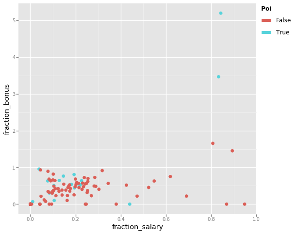
Intuitively I’d expect many of the persons of interest involved in the Enron scandal to have large contributions to their total payment from either a bonus or from some other means. In the scatter plot above you can see that many of the persons of interest receive a low salary in respect to their overall total payment but tend towards receiving a higher bonus. That is with exception to a small handful of Enron employees. Suspiciously there are a few data points that indicate a bonus much larger than the total payment they received. I thought this to be an error in the data, but having gone back to the FindLaw report it is clear that the total payment reported for some employees was significantly reduced due to deferred income.
Similarly I have plotted the salary as a fraction of total payment against long term incentive as a fraction of total payment.
ggplot(enron_data, aes(x='fraction_salary', y='fraction_long_term_incentive', color='poi')) + \
  geom_point(size=40.0)
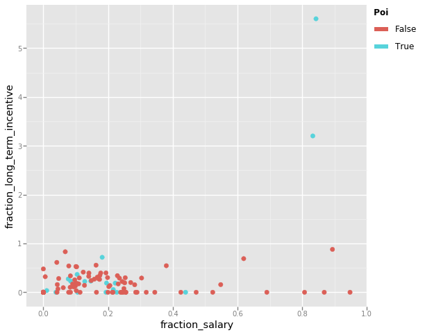
Apart from the two glaring obvious persons of interest that have long term incentives much larger than their total payment, there does not appear to be any conclusive trend in this data. However I shall keep this feature in case it proves useful to the classifiers. If I find this to not be the case this feature will likely be removed in the feature selection part of the experiment.
Next I’ll create a new stock value feature that, not too dissimilar to the new payment features, will represent exercised stock options as a fraction of the total stock value for each Enron employee. The rationale behind this new feature is that employees involved in the scandal may have been given huge amounts of stock that could be later sold.
I did not have any other feature that I though appropriate to plot this against so I’ll just leave this feature for the classifiers to judge it’s usefulness whilst performing feature selection.
enron_data['fraction_exercised_stock_options'] = enron_data.exercised_stock_options / enron_data.total_stock_value

# Replace any infinate or missing values.
enron_data = enron_data.replace([np.inf, -np.inf], np.nan)
enron_data = enron_data.fillna(0)
Last, I created new email features that attempt to tease out the frequency at which persons of interest were in contact (via email) with each other as a proportion to the total number of message they either sent or received. The reason I find these features to be of interest is because it seems likely for this scandal to have gone unnoticed for so long that key individuals were privately sending messages to coordinate fraudulent activity. More specifically I have created 2 new features:
- messages sent to a person of interest as a fraction of total messages sent
- messaged received from a person of interest as a fraction of total messaged received
I have plotted these two features against each other to find any trends.
enron_data['fraction_from_poi_to_this_person'] = enron_data.from_poi_to_this_person / enron_data.to_messages
enron_data['fraction_from_this_person_to_poi'] = enron_data.from_this_person_to_poi / enron_data.from_messages

ggplot(enron_data, aes(x='fraction_from_poi_to_this_person', y='fraction_from_this_person_to_poi', color='poi')) + \
  geom_point(size=40.0)
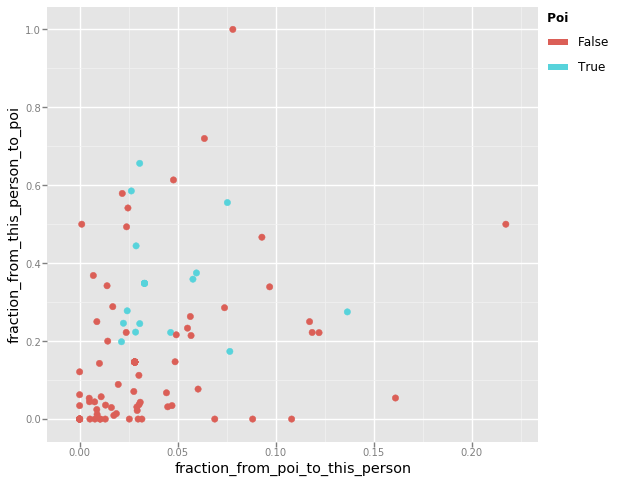
Intuitively I would have imagined persons of interest to sit somewhere towards the top right of the graph whilst the other employees would be scattered about as they innocently get on with their jobs. However the scatter plot does not contain any discernible pattern that I can see. What is apparent from this plot is that Enron employees tended to send more email messages to persons on interest than receive them.
However all is not lost as there are a few data points in this plot worth exploring. An interesting data point is the Enron employee that has not be flagged as a person of interest but has only ever sent email messages to other persons of interest. Lets find out who this is.
enron_data.sort_values(by='fraction_from_this_person_to_poi', ascending=False) \
  .loc[:, ['fraction_from_this_person_to_poi', 'from_messages']] \
  .head(2)
| fraction_from_this_person_to_poi | from_messages | |
|---|---|---|
| HUMPHREY GENE E | 1.00 | 17.00 |
| SHERRICK JEFFREY B | 0.72 | 25.00 |
Whilst I could not find much on the internet that would identify the role Gene Humphrey had at Enron I was able to discover to whom he was sending the messages:
- Kenneth Lay
- Jeffrey Skilling
Considering he only sent 17 messages it is not too hard to believe why this metric is so high.
Jeffrey Sherrick in another interesting data point who sent email messages primarily to Kenneth Lay. However this is justified by the fact he was the President of Enron Global Exploration & Production Inc. and therefore part of the corporate leadership and central management at Enron.
The last data point I want to explore is the employee that has clearly received the most emails from persons of interest as a fraction of the total number of emails received. Lets find out who this is.
enron_data.sort_values(by='fraction_from_poi_to_this_person', ascending=False) \
  .loc[:, ['fraction_from_poi_to_this_person', 'fraction_from_this_person_to_poi', 'to_messages', 'from_messages']] \
  .head(1)
| fraction_from_poi_to_this_person | fraction_from_this_person_to_poi | to_messages | from_messages | |
|---|---|---|---|---|
| DONAHUE JR JEFFREY M | 0.22 | 0.50 | 865.00 | 22.00 |
Jeffrey Donahue held a number of senior corporate development roles whilst at Enron and it is evident from the above table that 50% of the messages he sent were to a person of interest (which is only 11 messages). Additionally he received 190 messages from persons of interest, making up 22% of the messages he received overall. Taking a look at his email data I can see that he both sent messages to and received messages from the following persons of interest:
- David Delainey
- Kenneth Lay
- Jeffrey Skilling
So although neither Gene Humphrey, Jeffrey Sherrick nor Jeffrey Donahue are themselves persons of interest it is fascinating to discover that they were all in contact with the same few employees of the company involved in the scandal.
As before I will extract a dictionary from the dataframe we’ve been using
throughout this investigation, now including the new engineered features, and
reorient the data. In addition I will now be using the test_classifiers method
I implemented earlier to more comprehensively evaluate a list of classifiers
sequentially, and will continue to take this approach from this point in the
experiment.
engineered_features = [
  'fraction_salary',
  'fraction_bonus',
  'fraction_long_term_incentive',
  'fraction_exercised_stock_options',
  'fraction_from_poi_to_this_person',
  'fraction_from_this_person_to_poi'
]

# Append the engineered features to our list of original features.
extended_features_list = features_list + engineered_features

# Extract the data from the dataframe, including the engineered features.
my_extended_dataset = enron_data.to_dict(orient='index')

# Create a list of classifiers to evaluate.
clfs = [
  (u'Naive Bayes', GaussianNB()),
  (u'SVM', LinearSVC(C=1000.0)),
  (u'Random Forest', RandomForestClassifier()),
  (u'AdaBoost', AdaBoostClassifier())
]

test_classifiers(clfs, my_extended_dataset, extended_features_list)
=====> Running Naive Bayes

=====> Running SVM

=====> Running Random Forest

=====> Running AdaBoost
| accuracy | precision | recall | f1 | f2 | |
|---|---|---|---|---|---|
| AdaBoost | 0.87 | 0.56 | 0.47 | 0.52 | 0.49 |
| Random Forest | 0.88 | 0.68 | 0.30 | 0.42 | 0.34 |
| Naive Bayes | 0.76 | 0.25 | 0.36 | 0.30 | 0.33 |
| SVM | 0.73 | 0.22 | 0.36 | 0.27 | 0.32 |
The above table shows that overall adding these 4 new features has not had a
significant impact on the performance of each classifier, with exception to the
RandomForestClassifier that has an improved F1 score of 41% (an 8% increase).
This is due to both an increase in the precision and recall of this particular
classifier. This I admit is a little disappointing as I had hoped some latent
patterns to be discovered in these new features that would show a greater
performance across all the classifiers. However I will keep all of these
features until later feature selection deems them as having no significant
effect.